A few months ago, I saw this video of George Monbiot angrily pleading his case against perpetual growth and the lies of so-called, "green capitalism". At the beginning of his demonstration, he explains how the search for a modest rate of 3% growth in our economy leads to a doubling of production every 24 years. This made me think of a quote by the late professor of physics Albert Bartlett:

The greatest shortcoming of the human race is our inability to understand the exponential function.

— Albert Bartlett

In this post, I will try to contribute to the solution of this problem by providing my own interpretation of the exponential function and its meaning.

The mathematical definition of the exponential is the solution to the following problem:

Find the expression of a function proportional to its rate of growth

In mathematics, the rate of growth of a function $y(t)$ is equal to its first derivative, so that the above statement translates to:

$$
\begin{equation}
\frac{dy}{dt}=\lambda y(t)~,\label{eq:dydtexp}
\end{equation}
$$

where $\lambda$ is some constant of proportionality. Students of mathematics learn to solve the above equation in their first year of university. The result is

$$
\begin{equation}
y(t)=y(0)~e^{\lambda t}~,\label{eq:y(t)exp}
\end{equation}
$$

where $y(0)$ represents the value of the function at $t=0$. The real number $e\approx2.718$ is a fundamental constant, on par with other numbers like $\pi$.

The plot below shows the shape of Eq. \eqref{eq:y(t)exp} for $y(0)=1$ and for different values of $\lambda$. You can see that this parameter sets the steepness of the curve, the larger the steeper.

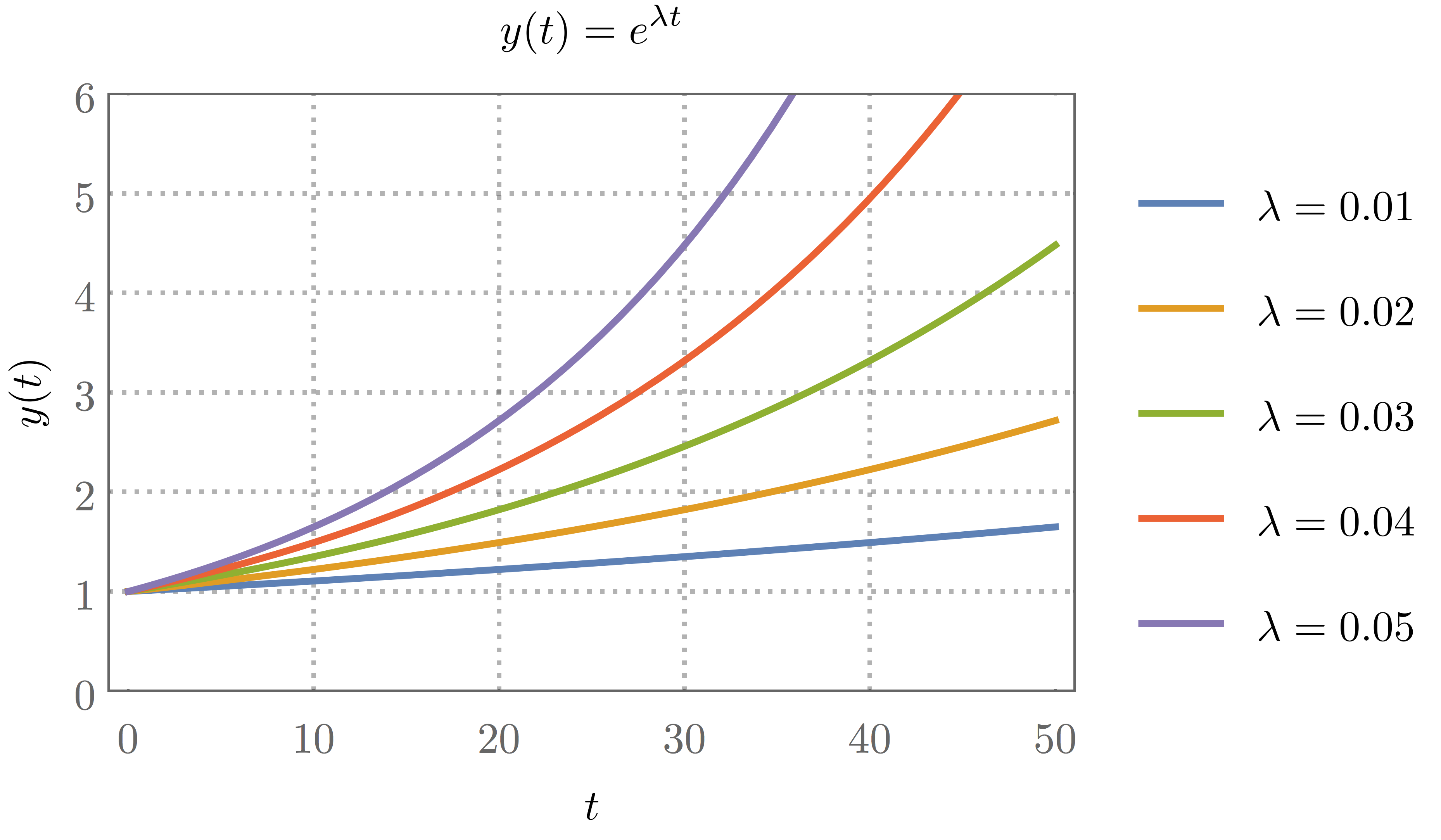
Now, perhaps the main source of confusion comes from the fact that $\lambda$ is what economists call the growth rate while for mathematicians, this name is employed to denote $dy/dt$ itself. From Eq. \eqref{eq:dydtexp}, we see that $\lambda$ is equal to the ratio $(dy/dt)/y(t)$, so that $\lambda$ could be more appropriately called the relative growth rate.

Using the above figure, we can understand a number of things. First of all, suppose that the x-axis represents time measured in years and that the y-axis represents the GDP of a country. By looking at the green curve, we can see that it checks out with George Monbiot's computation predicting a doubling of the economy every 24 years for a relative growth rate of 3%. In order to get the exact result, we can go back to Eq.(2), pose $y(t_2)=2y(0)$ and solve for $t_2$. This gives:

$$
\begin{align}
e^{\lambda t_2}&=2\\
t_2&=\frac{\text{ln}~2}{\lambda}
\end{align}
$$

which, for $\lambda=0.03$, gives $t_2\sim23.105$. The quantity $t_2$ is called the half-time constant from its usage in the study of the decay rate of radioactive materials where the exact same mathematics applies, except that the exponential is decreasing, corresponding to a negative value of $\lambda$.

The other thing to learn from the above figure concerns the limits to our intuition in relation to the idea of perpetual growth.

When economists talk about growth, they give a number in % per year and this is excatly what $\lambda$ stands for. However, as we are not used to that sort of vocabulary, we tend to mistake this quantity for the actual growth rate $dy/dt$ which measures the increase of a certain amount of currency (or material, or some other thing depending on the problem at hand) with time. By going back to Eq. \eqref{eq:dydtexp}, we can appreciate the difference between those two quantities. Even when $\lambda$ remains constant, the actual growth rate increases in proportion to the amout already accumulated. And since this amount increases continuously, accumulation becomes quicker and quicker as time goes by.

"Why aren't we able to visualize all of this more easily?" one might ask. We can answer that question by expanding Eq. \eqref{eq:y(t)exp} in series around $t=0$:

$$
\begin{equation}
y(t)=y(0)\left(1+\lambda t+\frac{(\lambda t)^2}{2!}+\frac{(\lambda t)^3}{3!}+...\right)~.
\end{equation}
$$

For $\lambda t<1$, the terms of the series become smaller with increasing powers. It is only after a sufficient amount of time has passed, when $t\approx1/\lambda$, that the terms of higher power start to dominate over those of smaller power and we can appreciate the exponential nature of growth. This is the reason why the blue curve, corresponding to the smaller value of $\lambda$ in the figure looks like a straight line until well after the other curves have stopped from doing so.