We are currently living through the coronavirus crisis (covid-19). A lot of people have tried to share a little insight on the mechanisms at play in the control of the epidemic and their mathematical modelling. Here, I would like to share a few things I have learnt recently on the subject. I want to insist that I am not an expert in epidemiology and so I do not recommend to use anything that follows as a basis of any decision. I merely want to outline the very broad principles involved in the mathematical modelling of epidemics.

I will focus specifically on the simple SIS and SIR models. This is based on the resolution of non-linear differential equations giving the proportion of people in a population that have been infected by the disease, $i(t)$, those who have not, $s(t)$ and those who have been infected but recovered $r(t)$. Let us assume first that the people who have been infected do not develop long-lasting immunity after they are cured. This implies that the recovered people count as susceptible people. Hence the total number of people are distributed among two compartments $s\leftrightarrow i$ . The equations are then:

$$
\begin{align}
\frac{ds}{dt}&=-\beta si+\gamma i~,\label{eq:dsdtSIS}\\
\frac{di}{dt}&=+\beta si-\gamma i~.\label{eq:didtSIS}
\end{align}
$$

In a previous post about exponential growth, we have seen how differential equations like those above define a relationship between functions and their rates of change. The situation here follows the same logic, except that there are now two functions rather than one. The first term of the right-hand side of each equation expresses the fact that the fraction of new infected patients is proportional to the number of persons already infected and to the number of persons that are not and so are susceptible to be. The last term of each equation takes into account the fraction of the infected people that become healthy again. The values of the two real parameters, $\beta$ and $\gamma$ dictates the behaviour of the epidemic. This is perhaps better understood by combining the Eq. \eqref{eq:dsdtSIS} and \eqref{eq:didtSIS} into a single one. In order to do so, we must first realize that the two add up to zero, so that the total number of people remains constant at all time:

$$
\begin{align}
\frac{d}{dt}(s+i)&=0~,\\
\leftrightarrow s+i&=k~.\label{eq:s+i=k}
\end{align}
$$

It is convenient to set the constant $k=1$ so that $s$ and $i$ are numbers between $0$ and $1$. Reinjecting Eq. \eqref{eq:s+i=k} into Eq. \eqref{eq:didtSIS} we arrive at :

$$
\frac{di}{dt}=(\beta-\gamma)i-\beta i^2~.
$$

This is a particular example of the logistic differential equation. If we ignore the second term on the right-hand side for a moment and compare what remains with our well-known equation for the exponential growth, we can identify the combination $(\beta-\gamma)$ as the growth rate. There are two possible behaviours: either $\beta>\gamma$ and so the solution grows exponentially, or $\beta<\gamma$ and the solution decays exponentially in time. Either of those two behaviours dominates when $i$ is small. When $i$ approaches $1$, the decaying effect of the second term kicks in and dominates over the first term. The two behaviours are represented on the following figure.

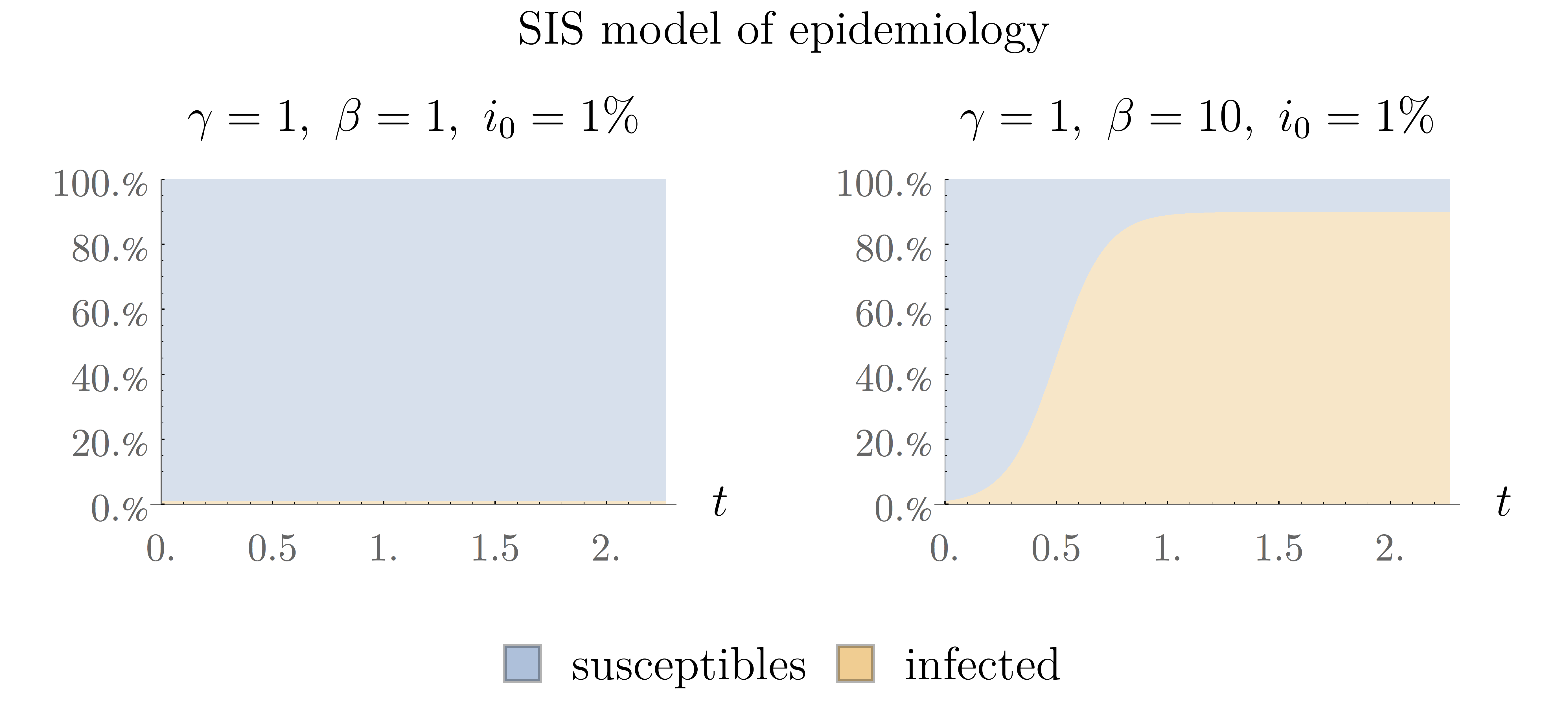
The area in orange represents the fraction of infected people in the population over time and the area in blue represent the fraction of the population that are not infected and are susceptible to be. In both cases, the fraction of infected people starts at $i_0=1%$. On the left plot, the number of infected decays very rapidly from the start so that the blue area clearly dominates at all time. On the right plot, the number of infected people grows very rapidly at first and then reaches a kind of equilibrium between the patients that are susceptible and those that are infected. This equilibrium happens when the flux of newly infected people is equal to the flux of people that become cured, i.e. when $\beta is=\gamma i$, or equivalently:

$$
\beta =\frac{\gamma}{s}\leftrightarrow R_0=\frac{1}{s}~,
$$

where we have defined $R_0\equiv\frac{\beta}{\gamma}$ . This last parameter is known as the basic reproduction number and is one of the most fundamental quantities in epidemiology as we will see shortly.

Having considered the simple SIS model in some details, we are now ready to tackle the more sophisticated SIR model. This differs to what precedes in the fact that now we have to look at three equations governing the dynamics of the population between three compartments:

$$
\begin{align}
\frac{ds}{dt}&=-\beta si~\label{eq:dsdtSIR}\\
\frac{di}{dt}&=+\beta si-\gamma i~,\label{eq:didtSIR}\\
\frac{dr}{dt}&=+\gamma i~.\label{eq:drdtSIR}
\end{align}
$$

The major difference with Eqs. \eqref{eq:dsdtSIS} and \eqref{eq:didtSIS} is that, now, people that have been infected and then cured, do not go back to the group of susceptible people but rather populate the set of recovered people. Because $\beta$, $\gamma$, $s$ and $i$ are all positive numbers, Eq. \eqref{eq:s+i=k} tells us that the fraction of the recovered can only go up in time while the fraction of the susceptible always goes down.The relation between the compartments can be summarized by $s\rightarrow i \rightarrow r$. Contrary to the SIS model, there is no way to reduce the dynamics to a single equation. The best we can do is to use $s+i+r=1$ to write Eqs. \eqref{eq:dsdtSIS} and \eqref{eq:didtSIS} in the following form:

$$
\begin{align}
\frac{ds}{dt}&=-R_0\gamma si~,\\
\frac{di}{dt}&=(R_0 s-1)\gamma i~,
\end{align}
$$

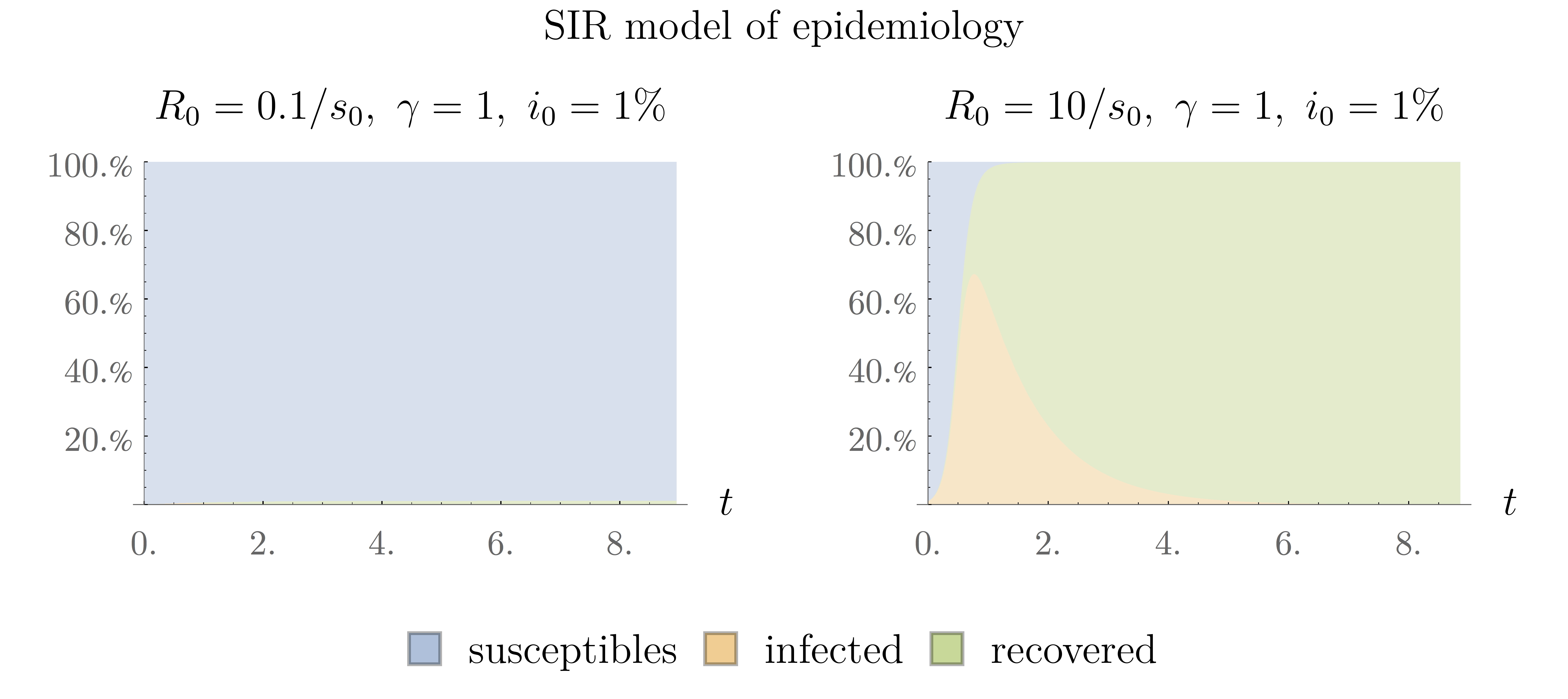
where we have inserted the definition of $R_0$. The value of this quantity at the beginning of the epidemic determines its dynamics, as we can see on the following figure:

{: .align-center}

On the left, we can see the situation when $R_0=\frac{0.1}{s_0}$, where $s_0$ represents the fraction of susceptible patients at initial time. In such case the people that are infected quickly recover, after what they cease to be infection and the number of cases remains small. The situation on the right is quite different. In that case, we have $R_0=\frac{10}{s_0}$, which means that people become infected more quickly than they recover and we end up with a proper epidemic. The threshold between those two regimes corresponds to $R_0=\frac{1}{s_0}$.

At the moment of writing this note, we are in the middle of a global epidemic of covid-19. A recent estimate heard on the radio mentions that half of the worldwide population lives currently isolated. We are obviously faced with a very infectious disease. We can sometimes see on the news that the isolation measures aim to flatten the curve. This statement can be understood by considering the effect that isolation has on the value of $R_0$. We have seen that this parameter depends on both $\beta$ and $\gamma$. The latter of which represents the rapidity with which people recover from the illness. It is perhaps easier to understand if we identify $\tau_R=\gamma^{-1}$ as the typical time before recovery. It is typically very difficult to influence this parameter except by significantly improving the care provided to patients or by inventing a new drug or vaccine. At any rate, such changes in $\gamma$ usually take a lot of time. It is more straightforward to influence the value of $\tau_C=\beta^{-1}$ which represents the typical time between transmissions of the virus from one infected to one susceptible person. Having people stay at home increases this time of contact and thus reduces $\beta$ and so $R_0$. The effect can be seen on the following animated figure.

We can see that the peak of the epidemic gets lower and lower as $\beta$ decreases. There are clearly two scenarios possible. If we manage to keep the curve very flat, the percentage of the population that is infected remains relatively small at all time. It can even be so low that most people get through the epidemic without ever being infected. On the other hand, if we are unable to flatten the curve, the number of infected patients can go very high, after what the number of susceptible people approaches zero rapidly indicating that most people have become infected and recovered and so the epidemic dies out. A situation called herd immunity.

Now, it is very important to bear in mind that there are a great deal of aspects that the very simple model above does not take into account. Crucially, by considering the total population as a constant we have always implicitly assumed that you cannot die from the disease regardless of the maximum number of people infected at once. This is obviously not true for an epidemic such as covid-19 which has proved to be very dangerous in many cases so that the survival rate of the population really depends on the capacities of the healthcare system which are obviously finite. Another thing that we did not consider is the possibility that after a short period of immunity following recovery, people become susceptible to become ill again. Such complex dynamics can be accommodated with more sophisticated models of epidemiology.

To conclude this note, I strongly encourage you to have a look at this video if you haven't already. It deals in the SIR model in considerably more details than I did here. Regarding the covid-19 epidemic specifically, I recommend this note as well as this paper which raises many issues regarding the relevance and the ethical implications of some of the measures that could be implemented to control the epidemic in the long run.