One important aspect of General Relativity is the computation of geodesics from a given metric of space-time. I will go through the details of how it can be done using the Riemann package.

Before tackling the space-time problem, let's warm up a bit and look at a simpler example in two-dimensional space.

1. Space

We will consider the following line-element:

$$
ds^2=\frac{dr^2}{(1-\frac{r_s}{r})}+r^2d\phi^2~,
$$
where ${r,\phi}$ are the usual polar coordinates. The parameter $r_s$ is analogous to the Schwarzschild radius. In a complete space-time computation, this is proportional to the mass at the centre of coordinates.

The geodesics are curves satisfying the following general equation
$$
\frac{d^2x^\alpha}{d\lambda^2}+\Gamma^\alpha_{\beta\gamma}\frac{dx^\beta}{d\lambda}\frac{dx^\gamma}{d\lambda}=0~.
$$
where ${x^\mu}_{\mu=1,..,d}$ denotes the set of coordinates of space considered to be functions of a single affine parameter $\lambda$ thus describing a family of one-dimensional curves. The $\Gamma$s are the Christoffel symbols. We are using Einstein's convention whereby repeated indices imply that there is a summation on those indices.

For our surface, the equations of geodesics are :
$$
\begin{array}{c}
r''(\lambda )+\frac{r_s r'(\lambda )^2}{2 r_s r(\lambda
)-2 r(\lambda )^2}+\phi'(\lambda )^2 (r_s-r(\lambda ))=0 \
\phi''(\lambda )+\frac{2 \phi'(\lambda ) r'(\lambda )}{r(\lambda)}=0
\end{array}
$$

The analytical resolution of these equation needs not concern us at the moment. For purposes of illustration, we can be content with a numerical resolution. In the notebook from the git repository, I define some simple initial conditions

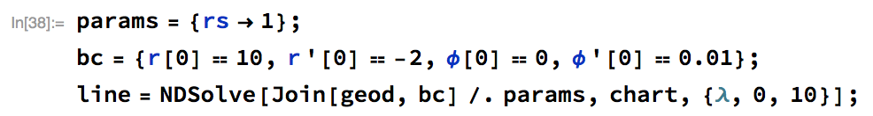
and plot the result as a parametric curve. Anticipating on the computation in space-time, we can plot our result curve on the Flamm's paraboloid representing the following embedding in 3d space:
$$
{x = r \cos (\phi ),~y = r \sin (\phi ),~z = 2 \sqrt{r-1}}
$$
The function Embedding3D in the preamble to the notebook has been written to serve that visualisation purpose. The geodesic is shown in blue:

2. Space-time

In order to take gravity into account, one must consider the complete space-time metric and restore the time coordinate:
$$
ds^2=-\left(1-\frac{r_s}{r}\right)dt^2+\frac{dr^2}{(1-\frac{r_s}{r})}+r^2d\theta^2+r^2\sin(\theta)^2d\phi^2~,
$$
where ${t,r,\theta,\phi}$ are the combination of time and usual spherical coordinates.

In this case, the geodesic equations are:
$$
\begin{align}
t''(\lambda )-\frac{r_s r'(\lambda ) t'(\lambda )}{r_s r(\lambda )-r(\lambda )^2}=0& \\
r''(\lambda )+\frac{r_s r'(\lambda )^2}{2 r_s r(\lambda)-2 r(\lambda )^2}+\theta'(\lambda )^2(r_s-r(\lambda ))+&\\
\sin^2(\theta (\lambda )) \phi'(\lambda )^2 (r_s-r(\lambda))+\frac{r_s(r(\lambda )-r_s) t'(\lambda )^2}{2r(\lambda )^3}=0& \\
\sin (\theta (\lambda )) \cos (\theta (\lambda )) \phi'(\lambda)^2-\theta''(\lambda )-\frac{2\theta'(\lambda ) r'(\lambda)}{r(\lambda )}=0& \\
2 \theta'(\lambda ) \cot (\theta (\lambda )) \phi'(\lambda )+\phi''(\lambda )+\frac{2\phi'(\lambda ) r'(\lambda )}{r(\lambda )}=0&~.
\end{align}
$$
We can solve these numerically as we did for the purely spatial case. There is however an extra subtlety here as one must not fail to consider one extra constraint stemming frome the principle of equivalence of general relativity. We will first address the case where the particle has mass and then move on to the case of a massless particle.

massive particle

The equivalence principle states that, at any point (event) of space-time, the laws of motion must be reducible to those of special relativity by an adequate choice of local coordinates which corresponds to a free-falling frame of reference. In the case of a massive particle, this amounts to demand that
$$
\begin{equation}
ds^2=-d\lambda^2~,\label{eq:ds2=-dlambda2}
\end{equation}
$$
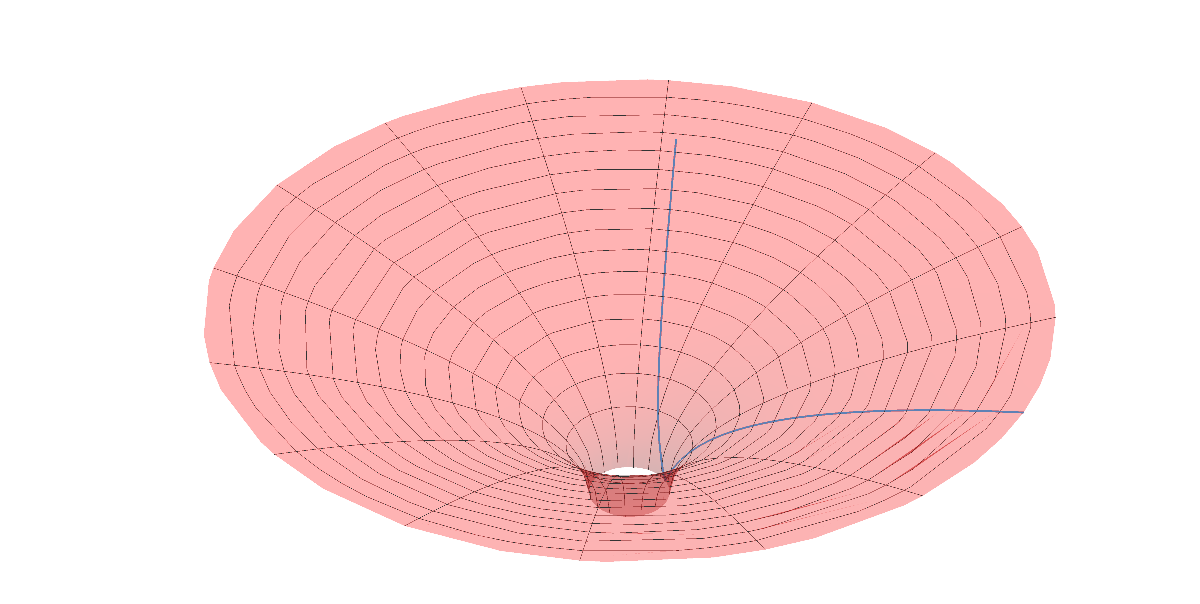
locally, where $\lambda$ is here interpreted as the proper-time of the particle. In practice, it means that, if one sets the initial value of all the coordinates functions $x^\mu(\lambda)$ and their derivatives except for $t'(\lambda)$, this latter quantity must be determined using Eq. \eqref{eq:ds2=-dlambda2}. Once everything has been set up properly, we can finally see some interesting physics taking place. Below is a plot of a trajectory in the equatorial plane. This corresponds to a particle starting at $r=10$ and with a very small azimuthal velocity $\phi'=\frac{1}{50}$ so it begins to orbit the centre of coordinates. The Schwarzschild's radius here is set to $r_s=1$.

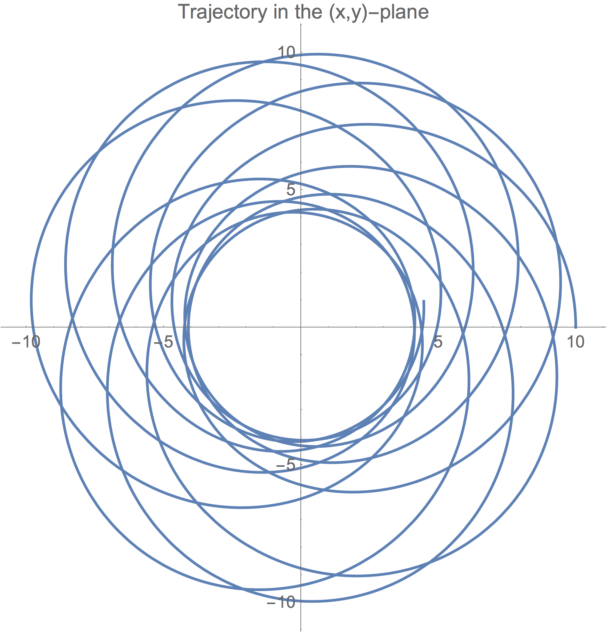
The figure below shows the same trajectory embedded on the surface of Flamm's paraboloid.

massless particle

The discussion on the choice of initial value presented above in the case of a massive particle needs to be modified when the particle has no mass.
Firstly, one must realise that the idea of proper-time is ill-defined for a massless particle and one must decide on another affine parameter to use. Perhaps the most natural choice is simply to use the element of length $\lambda=\ell$. Differentiating both sides with respect to $\lambda$ and taking the square leads to
$$
\begin{equation}
\left(\frac{d\ell}{d\lambda}\right)^2=1~,
\end{equation}
$$
which sets a contraint on the spatial part of the metric.
Another constraint comes from the fact that massless particle necessarily travel at the speed of light, which entails :
$$
\begin{equation}
ds^2=0~.
\end{equation}
$$
The above two constraints have to be satisfied simultaneously at all points of the trajectory.

The figure below shows one such trajectory in the equatorial plane for a particle starting at $r=5$ with a small initial radial velocity towards the centre $r'=-0.5$. The equivalence principle constrains the azimuthal velocity to $\phi'=\frac{\sqrt{1-r^{\prime 2}}}{r}$. We have chosen the value of the Schwarzschild's radius $r_s=\frac{5}{3}$.

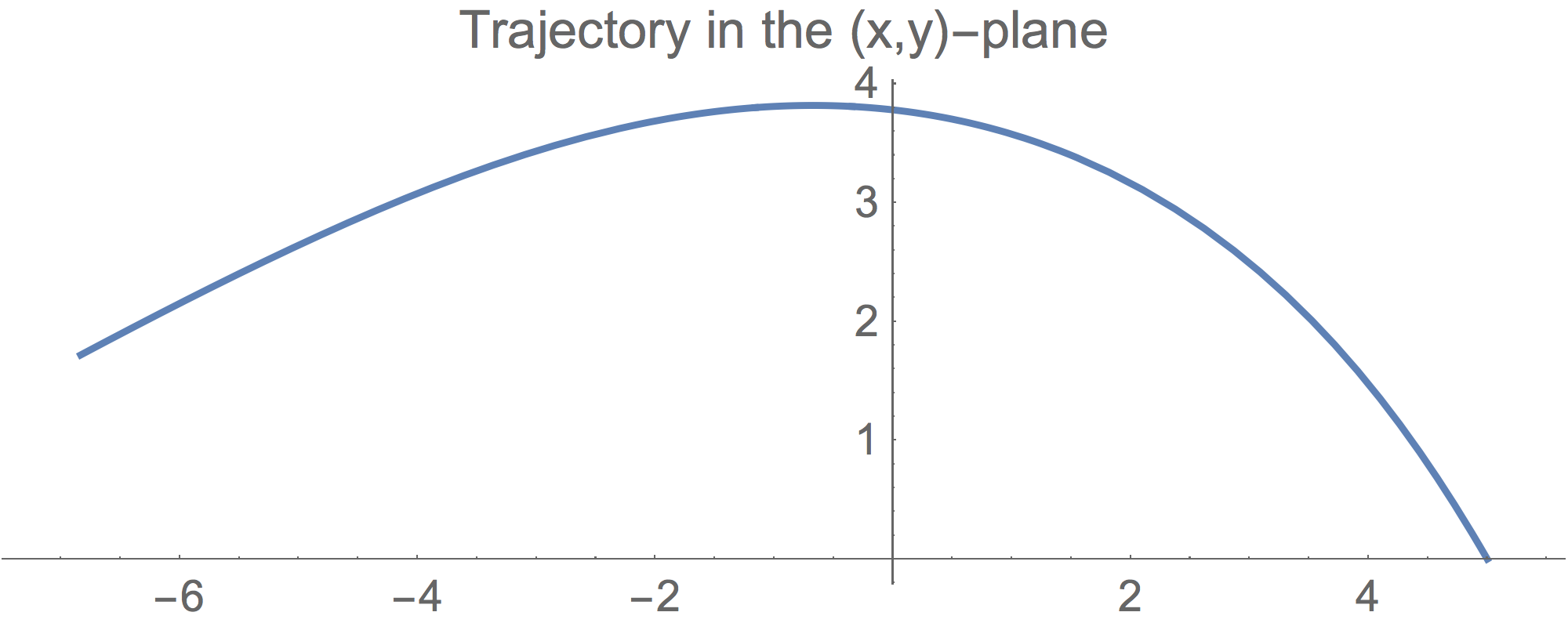
The above clearly demonstrates the effect of space-time curvature on the trajectories of a massless particle. It is perhaps the most stringent departure of general relativity from Newtonian physics that light rays are bent by gravitational fields.

In order to render that fact even more vividly, we can compare our results to that obtained by performing the same computation but setting the Schwarzschild's radius to $r_s=0$ thus effectively describing Minkowski's space-time. You will find both curves on the picture below embedded into the surface of Flamm's paraboloid.

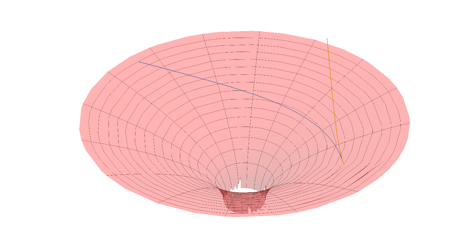
The blue curves is the solution for $r_s=\frac{5}{3}$, the yellow one is the one for $r_s=0$.