The most natural way of formulating Newton's laws of classical dynamics is to express the motion of particle relative to a frame of reference that is at rest (or has a constant velocity relative to some other frame). Such a frame is referred to as an inertial frame of reference. In some cases, however, it is easier to describe the motion relative to accelerated frames. Such is the case, for example, when one is interested in the motion of the atmosphere relative to the surface of the Earth, which is subjected to an acceleration caused by its diurnal rotation (the so-called centripetal acceleration).

In this post, I want to go back to basics and do a bit of point-particle mechanics in a frame rotating at a constant angular velocity.

In the absence of external forces, the Lagrange function is the kinetic energy of the particle with its total velocity written as a combination of its own velocity plus the contribution to the rotation of the whole frame:

$$
\begin{align}
L &= \frac{1}{2}m\left|~\dot{\vec{r}}+\vec{\omega}\times\vec{r}~\right|^2\\
&= \frac{1}{2}m\left|\dot{\vec{r}}\right|^2+m~\vec{\omega}\cdot\left(\vec{r}\times\dot{\vec{r}}\right)+\frac{1}{2}m\left[\omega^2r^2-(\vec{\omega}\cdot\vec{r})^2\right]
\end{align}
$$

We can set $~\vec{\omega}^{T}=\left(0,0,\omega\right)$ without loss of generality. In this case, the Lagrangian becomes

$$
L = \frac{1}{2}\left(\dot{x}^2+\dot{y}^2\right)+m\omega(x\dot{y}-y\dot{x})+\frac{1}{2}\omega^2(x^2+y^2)
$$

One sees that the motion is constrained to the $xy$-plane. The equations of motion are derived using the Euler-Lagrange equations. These give a system of first order differential equations that can be put in the following matrix shape :

$$
\begin{align}
\frac{d}{dt}
\left(
\begin{array}{c}
x\\
\dot{x}\\
y\\
\dot{y}
\end{array}
\right)=
\left(
\begin{array}{cccc}
0&1&0&0\\
\omega^2&0&0&2\omega\\
0&0&0&1\\
0&-2\omega&\omega^2&0
\end{array}
\right)
\left(
\begin{array}{c}
x\\
\dot{x}\\
y\\
\dot{y}
\end{array}
\right)
\end{align}
$$
The formal solution to the system is
$$
X(t)=e^{A[\omega]t}\cdot X(0)~,
$$
where $X(t)$ denotes the solution array and $A[\omega]$, the matrix on the right-hand-side of Eq.(1). The matrix exponential on the right-hand-side of the above is the propagator. Here is its full expression:
$$
\begin{aligned}
e^{A[\omega]t}=\scriptsize{
\begin{pmatrix}
\cos (\omega t)+\omega t \sin (\omega t) & t \cos (\omega t) & \sin (\omega t)-\omega t \cos (\omega t) & t \sin (\omega t) \\
\omega t^2 \cos (\omega t) & \cos (\omega t)-\omega t \sin (\omega t) & \omega t^2 \sin (\omega t) & \omega t \cos (\omega t)+\sin (\omega t) \\
\omega t \cos (\omega t)-\sin (\omega t) & -t \sin (\omega t) & \cos (\omega t)+\omega t \sin (\omega t) & t \cos (\omega t) \\
-\omega t^2 \sin (\omega t) & -\omega t \cos (\omega t)-\sin (\omega t) & \omega t^2 \cos (\omega t) & \cos (\omega t)-\omega t \sin (\omega t) \\
\end{pmatrix}}
\end{aligned}
$$

To better see the effect of this matrix, we can apply it to some initial conditions where the particle starts at the centre of coordinates with a unit velocity directed towards the x-direction: $X(0)^T=(0,1,0,0)$. The following figure illustrates the resulting motion. The trajectory is shown in blue and the velocity vector at different values of $t$ is shown in red.

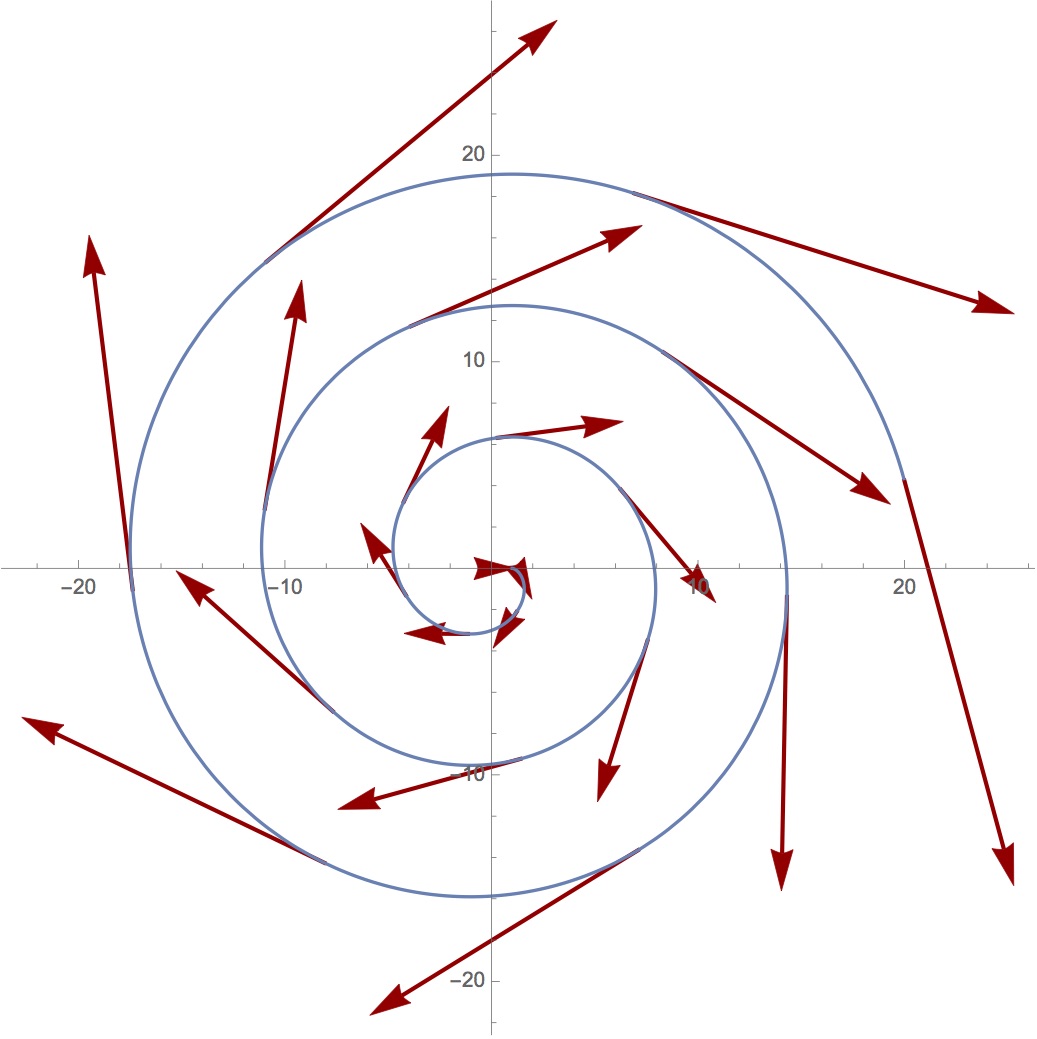
The figure was obtained after setting $\omega=1$ and solving from $t=0$ to $t=20$. Interestingly, one can see that the end position in the x-direction is 20, which is also the position that the particle would reach if it was moving in a straight-line along the x-direction with a constant unit velocity. This is what we would see from the inertial frame.

As a next exercise, we now find the initial conditions to reach the centre of coordinates from some outside point ($x_0,y_0$) after a time $t_c$ (central time). The solution reads

$$
\begin{align}
v_x^0&=-\frac{x_0-y_0\omega t_c}{t_c}\\
v_y^0&=-\frac{y_0+x_0\omega t_c}{t_c}
\end{align}
$$

One can understand these better by setting $y_0=0$. which give

$$
\begin{align}
v_x^0&=-\frac{x_0}{t_c}\\
v_y^0&=-\omega x_0
\end{align}
$$

The first of these is the mean velocity necessary to reach the centre in the time $t=t_c$. The second is the velocity necessary to counteract the velocity of rotation at a distance $x_0$ from the centre.

Setting $x_0=1$, the position vector of the particle reads

$$
\vec{r}=\left(1-\frac{t}{t_c}\right)\cos \omega t~\vec{e}_x - \left(1-\frac{t}{t_c}\right)\sin \omega t~\vec{e}_y
$$

We can write this vector in the inertial frame. The vector basis of the rotating frame {$\vec{e}_x$,$\vec{e}_y$} is related to the basis of the inertial frame {$\vec{X}$,$\vec{Y}$} via a rotation of angle $\omega t$ :

$$
\begin{align}
\left(
\begin{array}{c}
\vec{e}_x\\
\vec{e}_y
\end{array}
\right)=
\left(
\begin{array}{cc}
\cos\omega t & \sin\omega t\\
-\sin\omega t & \cos\omega t
\end{array}
\right)
\left(
\begin{array}{c}
\vec{X}\\
\vec{Y}
\end{array}
\right)
\end{align}
$$
which gives :
$$
\vec{r}=\left(1+v_x^0t\right)\vec{X}
$$
This is indeed the correct expression for a particle moving in a straight line with a constant velocity.

The next picture shows the comparison between the trajectory as seen from the rotating and inertial frames with the corresponding velocity vectors :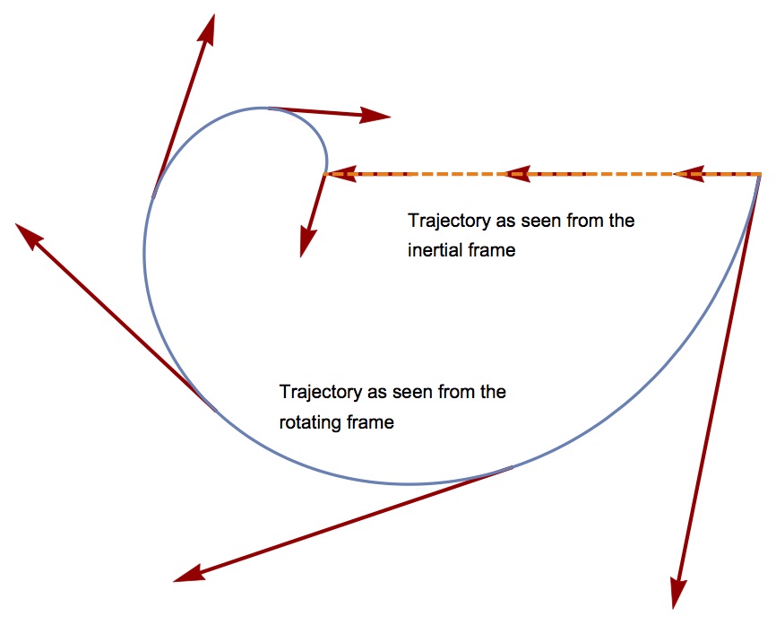

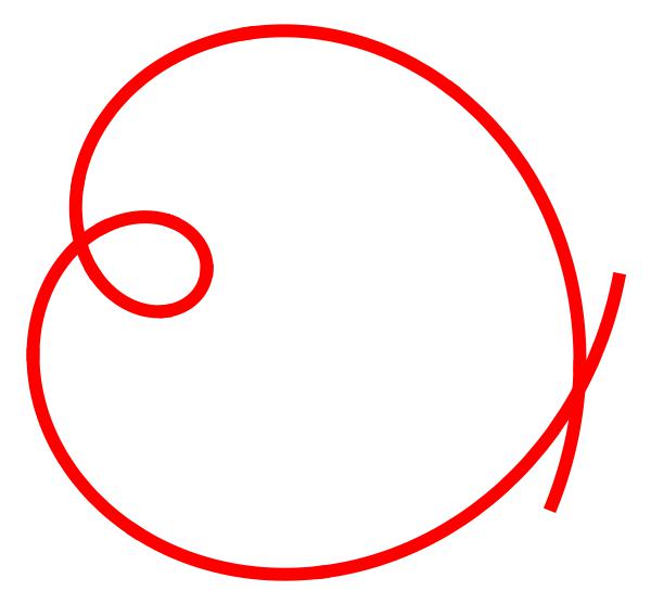
The velocity of the particle is not zero when it reaches the centre of coordinates so that it does not just stay in place.

The last picture shows the motion of the particle after it has reached the centre. Note that it is symmetrical and also a lovely way to close this post.